Predicting NBA lineup point differentials with ML
1. Project Description
In this project I gathered and clustered individual NBA player-seasons from 2000-2020 into 12 clusters using a gaussian mixture model with the goal of grouping together player-seasons with similar playing style (e.g. shot creation/selection/frequency), efficiency (e.g. true shooting percentage), and overall impact (e.g. box plus/minus). These clusters better represent the diverse functional roles that basketball players fill than the traditional 5 positions: point guard, shooting guard, small forward, power forward, and center. After identifying some interesting characteristics and league trends related to the clusters, I gathered NBA lineup data from 2000-2020 and attempted to predict lineup point-differentials per 100 possessions with a simple artificial neural network.
The inputs to the networks were lineup cluster profiles which were built by summing the player cluster labels across all players in a given lineup. The training targets were the observed lineup point-differentials per 100 possessions. Additionally, I attempted to predict lineup success with bpm-weighted cluster profiles that provide more information about the strengths and weaknesses of each lineup with respect to the clusters. The best performing network achieved a mean test error of around 5.6 points, a sizable error with respect to NBA lineup point differentials. All the data was scraped from the website basketball reference.
The code is available here.
Table of Contents
2. NBA Context
The NBA today is a fast moving landscape of player archetypes, player movement, team playing styles, and team-building strategies. Even the rules are changing with great rapidity as replay has become more available and players exploit the current boundaries of the game to hunt down advantages with increased focus and guile. Bruising big men are out, three pointers are in, defensive switchability is at a premium, championship equity is common parlance, and twitter burner accounts are the cherry on top of the most entertaining sports league.1 , 2
Many NBA front offices today are active experimenters, or at least willing followers of the innovators, in roster construction and player development. Having embraced new concepts, metrics, and aesthetics, teams trot out funky lineups, exploring different avenues to find any edge - including improved draft lottery odds.3 The willingness to explore the structure of basketball and build new mental models for thinking about the game is bound to continue uncovering competitive insights along with plenty of dead-ends.
As fans, how we watch and understand the game has been tugged along by the current of the game. We have been force-fed shot chart maps highlighting what a healthy shot diet consists in and now we grimace watching our favorite team's young star indulge in taking difficult deep 2-pointers;4 a habit of many stars of yesteryear. The previously niche lexicon of analytics has gradually wedged itself into a central role in our watching, understanding, and debating.
And yet at the core of things remain the traditional 5 positions, unchanged for decades, and continuing to passively frame our expectations, imagination, and understanding of basketball. Positions are the most common currency of description when discussing players and teams. Each position maps to a suite of functional roles and these boundaries help us to organize and chunk the game of basketball into manageable components when playing, coaching, evaluating, and watching. Positions are indeed necessary, but as with everything we should be aware of the role these concepts play in shaping our perspective on the very thing they purport to describe.
In the NBA today the best example of an over-discounted positional outlier is Ben Simmons. He is an elite defender, passer, and one-player transition engine, but he refuses to shoot from distance. His positive qualities make him an All-NBA player (i.e. roughly a top 15 player in the league). However, when his skills and weaknesses are combined in a single package, the sum elicits great confusion and his value is questioned. He falls far outside our established frameworks for understanding the game, and thus - to my mind - is underrated by many fans.
The influence of the positional hierarchy is far-reaching. For example, many who played basketball growing up are familiar with the lazy assignment of the smallest kid to point guard and the biggest kid to center. This pigeon-holing is common, and reveals a pervasive unthinking habit of mapping players to defined traditional roles solely based on height and stature. Real decision makers in the NBA must have sophisticated heuristics for understanding player roles and potential, but as fans it is time we to update our taxonomy of players to better reflect the playing style, efficiency, and value of players in the NBA today.
3. Building the Player Dataset
The first set of tasks was gathering the statistical data, cleaning it, combining it with other useful data, and transforming it to so that the combined dataset is easier to analyze and use with machine learning algorithms.
3.1. Scraping player-season stats & biographical data
I initially scraped data from nba.com/stats but switched to basketball reference. Basketball reference has all statistics I was hoping to make use of, as well as the convenient feature of using unique player ids throughout the site.5 These ids make it easy to verify and combine data from various areas on the site, such as player stats, player biographical information, and lineup data. I gathered four types of player statistics from the 1996-97 season through the 2019-20 season:
- advanced: e.g. box plus/minus, true shooting percentage, usage percentage
- shooting: e.g. percent of field goals taken from 0-3 feet away, percent of 3-pointers that were assisted
- play-by-play: e.g. percent of minutes spent at each traditional position, number of bad pass turnovers, total number of points generated by assists
- per 100 possessions: e.g. points/100 poss., free throws attempted/100 poss.
To scrape the data I used selenium to automate site navigation and expose the correct stat tables, beautiful soup to parse the html tables, and pandas to store the extracted data. The four stat types contained 88 distinct stat columns when combined on year and player ids to form a single player-season. To supplement these statistics I used the sportsreference api 6 to gather biographical data from basketball reference that included height, weight, salary, and nationality.
Scraping code
import time
from functools import reduce

import pandas as pd
from bs4 import BeautifulSoup
import selenium
from selenium import webdriver
from selenium.webdriver.common.action_chains import ActionChains
from selenium.webdriver.common.keys import Keys


def select_season(browser, season):
    "Navigate browser to the given season."
    url = f'https://www.basketball-reference.com/leagues/NBA_{season}_per_poss.html'
    browser.get(url)

def select_stat_table(browser, stat_table):
    "Navigate browser to the given statistic table. Current season must be 1995-96 onward."
    stat_table_dict = {'totals': 1,
                      'per_game': 2,
                      'per_minute': 3,
                      'per_poss': 4,
                      'advanced': 5,
                      'pbp': 6,
                      'shooting': 7,
                      'adj_shooting': 8}
    n = stat_table_dict[stat_table]
    button_xpath = f'/html/body/div[2]/div[5]/div[2]/div[{n}]/a'
    browser.find_element_by_xpath(button_xpath).click()

def read_stat_table(soup):
    "Parse the html table on the bs4 object's current page and return stats DataFrame."
    table = soup.find(class_="table_outer_container")
    tbody = table.find('tbody')
    tbody_tr = tbody.find_all('tr')
    stat_cols, all_stats, all_ids = [], [], []

    for row in tbody_tr:
        # skip partial rows i.e. player entries with multiple teams
        if row['class'] != ["full_table"]: continue
        cols = row.find_all('td')
        if stat_cols == []:  # extract stat names
            stat_cols = [col.get('data-stat') for col in cols]
        player_stats = [col.text for col in cols]  # extract player stat values
        all_stats.append(player_stats)
        player_id = cols[0].get('data-append-csv')  # extract unique player id
        all_ids.append(player_id)

    df = pd.DataFrame(all_stats, columns=stat_cols).set_index('player')
    df['player_id'] = all_ids

    return df

def process_scraped_table(df, season):
    "Drop redundant columns, add year column, update index. Return DataFrame."
    nunique = df.apply(pd.Series.nunique)
    drop_cols = nunique[nunique == 1].index
    df.drop(drop_cols, axis=1, inplace=True)
    df['year'] = [season] * len(df)
    df.index += f' {str(season)}'
    return df

def combine_season_stats(dfs):
    "Merge the stat tables from the same season on player ids."
    dfs = [df.reset_index().set_index('player_id') for df in dfs]
    season_df = reduce(lambda left, right: pd.merge(left, right[right.columns.difference(left.columns)], left_index=True, right_index=True), dfs)
    return season_df.reset_index().set_index('player')

def scrape(seasons, stat_types, data_dir):
    """
    Scrape player season stats from basketball reference for the given stat types
    across the given seasons and write out csv to given directory. Return DataFrame.
    """
    options = webdriver.firefox.options.Options()
    options.headless = True
    browser = webdriver.Firefox(executable_path="scraping/drivers/geckodriver", options=options)
    dfs = []

    for season in seasons:
        print('scraping:', season)
        season_dfs = []
        select_season(browser, season); time.sleep(3)

        for stat_type in stat_types:
            select_stat_table(browser, stat_type); time.sleep(3)
            page_source = browser.page_source
            soup = BeautifulSoup(page_source, 'html.parser')
            df = read_stat_table(soup)
            df = process_scraped_table(df, season)
            filename = data_dir + str(season) + '_' + str(stat_type).replace(' ', '_') + '.csv'
            df.to_csv(filename)
            season_dfs.append(df)

        combo_season_df = combine_season_stats(season_dfs)
        filename = data_dir + str(season) + '_' + '_'.join(stat_types) + '.csv'
        combo_season_df.to_csv(filename)
        dfs.append(combo_season_df)

    if len(seasons) < 2:
        return dfs[0]

    master_df = pd.concat(dfs)
    filename = data_dir + str(seasons[0]) + '_to_' + str(seasons[-1]) + '_' + '_'.join(stat_types) + '.csv'
    master_df.to_csv(filename)

    return master_df
Execute scraping:
from bball_ref_scraping_funcs import scrape

data_dir = 'nba_data/'
seasons = [year for year in range(1997, 2021)]
stat_types = ['advanced', 'shooting', 'pbp', 'per_poss']

if __name__ == '__main__':
    scrape(seasons, stat_types, data_dir)
3.2. Cleaning the data
At this point the raw player dataset had shape (11162, 92) with rows of individual player-seasons and stat columns. After imposing a minutes threshold of 650 minutes the dataset was reduced to (7363, 92). After filling in some straightforward NaNs I took a look at the remaining missing values to see if there were any anomalies in data collection:
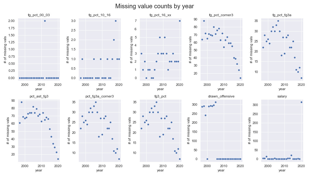
- Observations:
- Early
drawn_offensivedata is mostly missing - Salary information is missing for all of 2020 and for a few other rows throughout
- All other missing data is related to shooting percentages or shooting location
- Noticeable decrease in missing values for percentages related to 3-point shooting as more players began to shoot from deep in recent seasons
- Early
- Solutions:
- Drop
drawn_offensive - impute missing salary data with
"missing" - Verify missing shooting data and fill with 0s
- i.e. check that missing value for
fg_pct_00_03reflects that a player took 0 attempts from specified region and is not otherwise anomalous
- i.e. check that missing value for
- Drop
3.3. Transforming the data
To prepare the dataset for dimensionality reduction and clustering some further steps were taken:
- Drop seasons prior to 2000 given sketchy play-by-play data
- Remove some highly correlated stats (> 95% correlation)
- Log transform 22 columns
- Clip 3-point related percentages for very low volume 3-point shooting
players with outlier percentages to help differentiate great shooters
- e.g. Clip a player's 75% 3-point shooting percentage if it came on less than 1 3-point attempt per 100 possessions to better reflect the player's shooting ability
- Drop
yearandnationality - Scale with
sklearn.StandardScaler
ALL positive numeric initial stat distributions

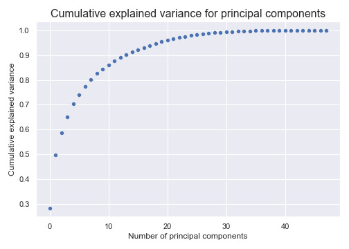
3.4. Principal component analysis (PCA)
After dropping some more columns (e.g. age, stats related to traditional positions, etc.) I used PCA to further transform the data into a more easily separable space and reduce the dimensionality from 48 dimensions to 29 dimensions while retaining 99% of the variance within the dataset.
4. Clustering
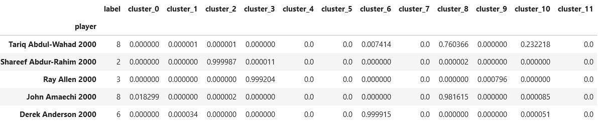
After experimenting with k-means and DBSCAN clustering I settled on using a gaussian mixture model (GMM) and expectation-maximization (EM) algorithm to generate 12 cluster probabilities for each player-season. The ability of GMMs to identify clusters with arbitrarily shaped densities and the nuance of probabilistic cluster labels, compared with hard cluster labels, were both attractive. However, most player-seasons belong to a single cluster with high probability. 7
Generate cluster labels (sklearn)
import pandas as pd
from sklearn.mixture import GaussianMixture

df = pd.read_csv('../datasets/pca99_2000_2020.csv', index_col=0)
seed = 3
n_comps = 12
gmm = GaussianMixture(n_components=n_comps,
                      covariance_type='full',
                      max_iter=10_000,
                      n_init=8,
                      random_state=seed)
gmm.fit(df)
hard_labels = gmm.predict(df)
soft_labels = gmm.predict_proba(df)
df_clusters = pd.DataFrame(hard_labels, index=df.index, columns=['label'])
soft_cols = [f'cluster_{n}' for n in range(gmm.n_components)]
df_clusters[soft_cols] = soft_labels
df_clusters.head()  # image below
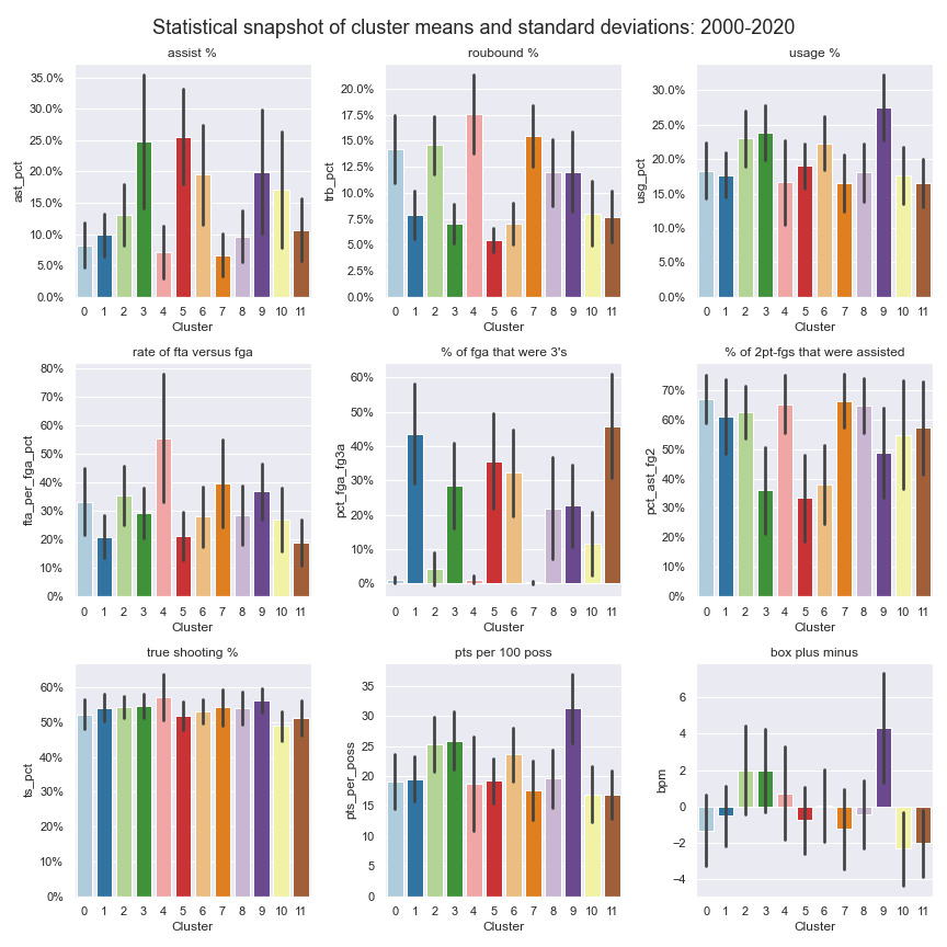
4.1. Clusters overview
All the statistical, biographical, pca, and cluster label datasets were combined into a single dataset to help isolate interesting features about the clusters. To begin differentiating them I looked for the major areas of statistical difference between and within clusters. Using plots like the one following the table below, I determined the defining features of each cluster and came up with representative names for each cluster which appear below.
| Cluster | Count | Name | Sample Seasons |
|---|---|---|---|
| 0 | 327 | Reserve Bigs | Enes Kanter 20', Tiago Splitter 14', Glen Davis 12, Tyrus Thomas 07' |
| 1 | 852 | Secondary Wings (3&D) | Jae Crowder 19', Shane Battier 14', Rick Fox 01', James Posey 00' |
| 2 | 241 | Effective Skilled Bigs | LaMarcus Aldridge 14', Chris Bosh 13', Pau Gasol 06', Vlade Divac 01' |
| 3 | 635 | Effective Lead Ball Handlers | Ja Morant 20', Chris Paul 12', Jameer Nelson 07', Jason Kidd 2002 |
| 4 | 142 | Traditional Centers | Hassan Whiteside 20', DeAndre Jordan 12', Dwight Howard 10', Ben Wallace 08' |
| 5 | 604 | Passing Offensive Initiators | J.J. Barea 19', Rajon Rondo 15', Luke Ridnour 08', Damon Stoudamire 03' |
| 6 | 635 | Scoring Focused Guards | Lou Williams 20', Nick Young 13', Jason Terry 09', Steve Francis 07' |
| 7 | 1,001 | Variety Post Bigs | Ed Davis 18', Joakim Noah 17', Kenneth Faried 13', Leon Powe 09' |
| 8 | 675 | Variety Wings & Stretch Bigs | Kelly Olynyk 19', Omri Casspi 15', Josh Childress 08', Gerald Wallace 06' |
| 9 | 326 | High Usage/Scoring/Impact Stars | LeBron James 20', James Harden 18', Tracy McGrady 05', Kevin Garnett 04', |
| 10 | 403 | Variety Ball handlers | Boris Diaw 17', Kyle Anderson 16', Shaun Livingston 14', Michael Beasley 13' |
| 11 | 703 | 3pt Specialists & Low-impact Reserve Wings/Forwards | Ben McLemore 20', Matt Bonner 11', Jason Kapono 11', Luke Walton 09' |
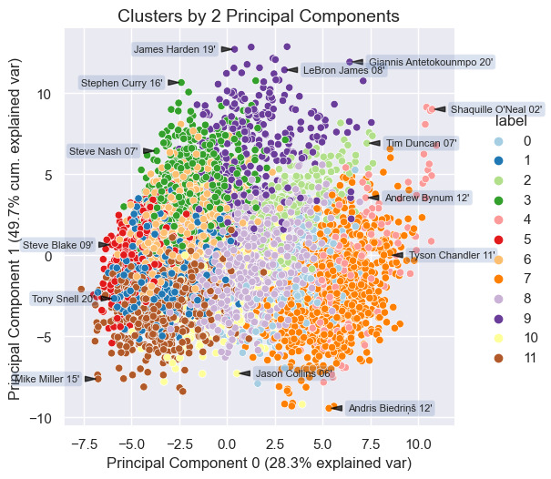
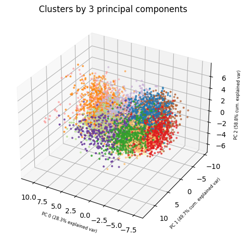
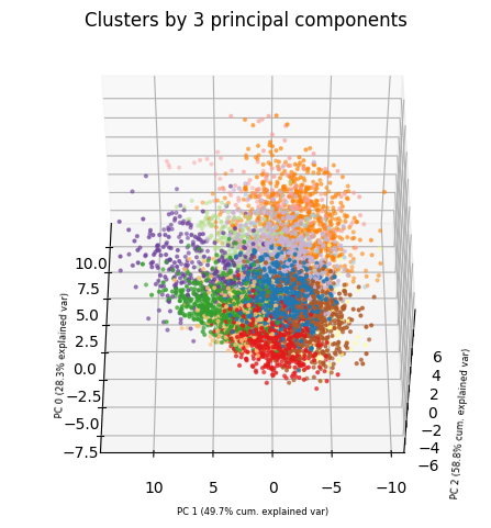
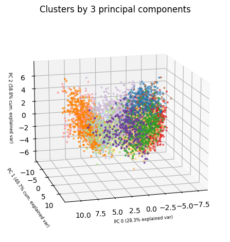
4.2. PCA plots to visualize cluster spacing
To get a rough visual intuition for the relative spacing of the clusters I plotted player-seasons according to their major principal components from the earlier PCA. Sizing the data points by box-plus minus provides further information about the box score impact that players from each cluster tend to have; principal component number 1 appears to have a near linear relationship with box-plus minus in the two-dimensional plot. The relative player-season spacing highlighted by the annotations makes intuitive sense to a basketball fan like myself. Polar opposite players such as Mike Miller and Shaquille O'Neal should be very widely spread out, and we do see that below.
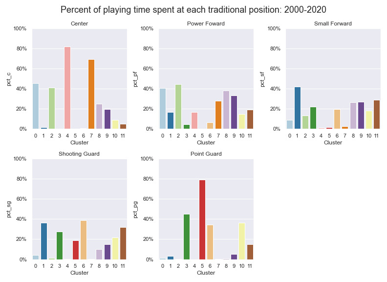
4.3. Clusters vs traditional positions
One of the first comparisons I looked into was the relationship between the clusters and the traditional positions. Using play-by-play data that provides the percentage of minutes a player plays at each traditional lineup position I compared how the clusters and traditional positions overlap. Below we see that only three clusters (4,5,7) spend a majority of their time at a single position. It is unsurprising that the strongest cluster and position relationships are between centers and point guards, as these two positions have the most differentiated set of roles among the five traditional positions. Still, centers and point guards are far from homogenous groups and both are well-represented across several clusters each.
4.4. Finances & player counts
Money talks, and in the NBA it speaks to which players NBA front offices value and believe contribute to winning basketball games. Contracts in the NBA are constrained by a soft spending cap on team spending each year, 8 as well as rules defining the minimum and maximum amounts that players at different stages of their career can earn. As the league changes, so to does the types of players who get paid the most.
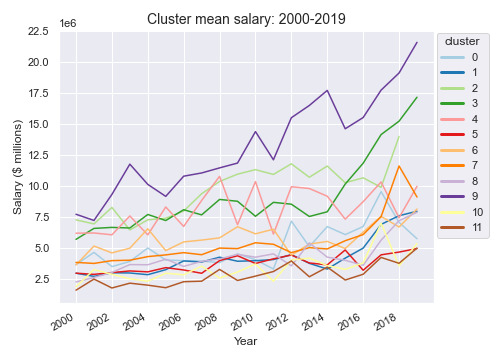
The growth of mean salaries for clusters 9 ("high impact stars") and 3 ("effective lead ball handlers) stands out when looking at the mean salaries for each cluster from 2000-2019. This mirrors the known trend towards versatile guards and wings and away from traditional post-centric offensive anchors. Clusters 9 and 3 are indeed composed of well-known and coveted players, and looking at the statistical snapshot from earlier we see that these two clusters are leaders in box plus/minus. Teams appear willing to pay more today for the most impactful players; current payrolls are more aligned with the conventional wisdom that the NBA is a star-dominated league.
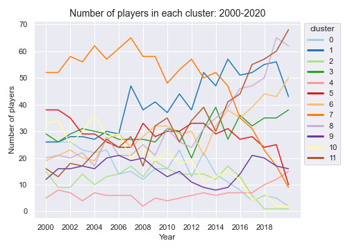
Looking at the number of players in each cluster by year we see further evidence for the demise of the traditional big man. Cluster 0 ("reserve bigs") and cluster 7 ("variety post bigs") have seen their numbers fall considerably in the last 20 years. However, there remains a solid contingent of "traditional centers" in the league even while the overall influence of post-bigs wanes; players like Hassan Whiteside and DeAndre Jordan. On the rise are clusters with positive shooting attributes: cluster 1 ("secondary wings (3&D)"), cluster 8 ("variety wings & stretch forwards"), and cluster 11 ("3pt specialists & low-impact reserve wings/forwards").
There are very few player-season representing cluster 10 ("variety ball handlers") and cluster 2 ("effective skilled bigs") in the most recent seasons. The types of player-seasons in these two clusters may simply not be well-represented in the modern NBA. For example, players who we may consider the next iteration of someone like Toronto Chris Bosh (cluster 2 and 9) almost definitely takes 3-pointers today and generally plays a game more tailored towards today's trends, perhaps precluding them from membership in cluster 2.
5. Lineup Analysis
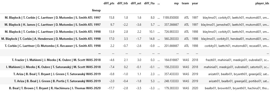
5.1. Scraping lineup data
To acquire the lineup data I turned again to basketball reference which maintains statistics for 5-player, 4-player, 3-player, and 2-player lineup combinations going back to the 1996-97 season. I gathered all the lineup data for every 5 and 4 player lineup from 1996-97 through 2019-20. One nuance in scraping the lineup data was the need to be aware of team name transitions and relocations given that the lineup data is housed within franchise pages. After scraping the data I immediately applied minutes thresholds of 150 for 5-player lineups and 300 for 4-player lineups. After adding some columns like number_players, team, year, player_ids to the lineup datasets, the initial datasets had shape (1964, 27) for 5-player lineups and (5977, 27) for 4-player lineups.
Lineup scraping code
def select_team_and_year_lineups(browser, team, year):
    "Navigate browser to given franchise page and year."
    url = f'https://www.basketball-reference.com/teams/{team}/{year}/lineups/'
    browser.get(url)

def read_lineup_table(soup, n_man_lineup):
    """
    Parse the html lineup stat table for the lineup type given by n_man_lineup
    (i.e. 4-player or 5-player lineups) on the current bs4 object page.
    Return DataFrame.
    """
    all_stats, all_lineup_ids, stat_cols = [], [], []
    table = soup.find('table', {'id': f'lineups_{n_man_lineup}-man_'})
    tbody = table.find('tbody')

    for row in tbody.find_all('tr')[0:-1]:
        cols = row.find_all('td')
        stat_cols = [col.get('data-stat') for col in cols]

        lineup_ids = [cols[0].get('csk')]
        all_lineup_ids.append(lineup_ids)

        lineup_stats = [col.text for col in cols]
        all_stats.append(lineup_stats)

    df = pd.DataFrame(all_stats, columns=stat_cols).set_index('lineup')
    df['player_ids'] = all_lineup_ids
    df['number_players'] = [n_man_lineup] * len(df)

    return df

def process_lineup_df(df, team, year):
    """
    Process the extracted lineup stat table:
      - Convert minutes played to numeric datatype
      - Fill blanks with NaNs
      - Convert differential stats to floats
      - Add year and team columns
      - Update index to reflect players, team, and year

    Return DataFrame.
    """
    df.loc[:, 'mp'] = df['mp'].apply(lambda x: float(x.split(':')[0]) + float(x.split(':')[1])/60)
    df.loc[:, 'player_ids'] = df['player_ids'].apply(lambda x: x[0].replace(':', ', '))
    df.replace('', np.nan)
    conv_to_float_cols = df.columns[df.columns.str.contains('diff')]
    df.loc[:, conv_to_float_cols] = df[conv_to_float_cols].apply(lambda series: pd.to_numeric(series, errors='ignore'))
    df['year'] = [year] * len(df)
    df['team'] = [team] * len(df)
    df.index = df.index + f' {team} {year}'

    return df

def scrape_lineup_data(teams, seasons, n_man_lineup, data_dir):
    """
    Scrape lineup data from basketball reference for given teams and seasons
    for the given lineup type (i.e. 4-player or 5-player lineups). Write out team
    lineup DataFrames and combined DataFrame to the given data directory.
    Return combined DataFrame.
    """
    options = webdriver.firefox.options.Options()
    options.headless = True
    browser = webdriver.Firefox(executable_path="scraping/drivers/geckodriver", options=options)
    start = datetime.now()
    all_dfs = []
    for team in teams:
        team_dfs = []
        print('scraping:', team, '   |   ', datetime.now()-start)
        for season in seasons:
            # handle team name switches etc.
            if team == 'NJN' and season > 2012: team = 'BRK'; print('Season:', season, '-->', team)
            if team == 'NOH' and season < 2003: continue # not a team prior to 2002-03
            if team == 'NOH' and season == 2006: team = 'NOK'; print('Season:', season, '-->', team)
            if team == 'NOK' and season == 2008: team = 'NOH'; print('Season:', season, '-->', team)
            if team == 'NOH' and season == 2014: team = 'NOP'; print('Season:', season, '-->', team)
            if team == 'SEA' and season > 2008: team = 'OKC'; print('Season:', season, '-->', team)
            if team == 'WSB' and season > 1997: team = 'WAS'; print('Season:', season, '-->', team)
            if team == 'CHH' and season > 2002: team = 'CHA'; print('Season:', season, '-->', team)
            if team == 'CHA' and season in [2002, 2003, 2004]: continue  # no charlotte team 2002-2004
            if team == 'CHA' and season > 2014: team = 'CHO'; print('Season:', season, '-->', team)
            if team == 'VAN' and season > 2001 : team = 'MEM'; print('Season:', season, '-->', team)

            select_team_and_year_lineups(browser, team, season)
            page_source = browser.page_source
            soup = BeautifulSoup(page_source, 'html.parser')
            df = read_lineup_table(soup, n_man_lineup)
            df = process_lineup_df(df, team, season)
            team_dfs.append(df)

        combined_team_df = pd.concat(team_dfs)
        filename = data_dir + f'{team}/{team}_{n_man_lineup}_man_lineups_{seasons[0]}_{seasons[-1]}.csv'
        os.makedirs(os.path.dirname(filename), exist_ok=True)
        combined_team_df.to_csv(filename)
        all_dfs.append(combined_team_df)

    df = pd.concat(all_dfs)
    filename = f'bballref_data/raw_all_teams_{n_man_lineup}_man_lineups_{seasons[0]}_{seasons[-1]}.csv'
    df.to_csv(filename)
    return df
Execute scraping:
from bballref_lineup_scraping_funcs import scrape_lineup_data

data_dir = 'bballref_data/lineups/'
n_man_lineup = 5
seasons = [year for year in range(1997, 2021)]
teams = [
        'ATL',
        'NJN',  # switches to BKN
        'BOS',
        'CHH',  # switches to CHA then CHO
        'CHI',
        'CLE',
        'DAL',
        'DEN',
        'DET',
        'GSW',
        'HOU',
        'IND',
        'LAC',
        'LAL',
        'VAN',  # switches to MEM
        'MIA',
        'MIL',
        'MIN',
        'NOH',  # switches to NOP
        'NYK',
        'SEA',  # switches to OKC
        'ORL',
        'PHI',
        'PHO',
        'POR',
        'SAC',
        'SAS',
        'TOR',
        'UTA',
        'WSB', # switches to WAS
        ]

if __name__ == '__main__':
    scrape_lineup_data(teams, seasons, n_man_lineup, data_dir)
5.2. Building lineup cluster profiles
Each lineup in the final lineup dataset has a cluster profile that is a summation of the individual cluster profiles of the players in the lineup. More than five clusters can be represented in each lineup given the soft probabilistic labels produced by the Gaussian Mixture Model. In addition to the straightforward lineup cluster profiles, I created bpm-weighted lineup cluster profiles. The bpm-weighted cluster profiles simply weight each player-season's cluster profile by the player-season bpm before adding it to the lineup cluster profile. The bpm-weighted cluster profile is meant to provide context about where a lineup's strengths and weaknesses lie with respect to the clusters.
Building the lineup dataset with cluster profiles requires 2 steps. First, verify the validity of each lineup with reference to the player dataset. Second, sum the cluster profiles of each player in a particular lineup and produce the lineup cluster profiles.
Functions for verifying and building lineup cluster profiles
def verify_players(lineup, df_players):
    """
    Return a boolean indicating whether all players in given lineup are
    present in the provided player dataset.
    """
    player_ids = lineup['player_ids'].split(', ')
    year = lineup['year']

    for pid in player_ids:
        if df_players[(df_players['year']==year) &
            (df_players['player_id']==pid)].empty:
            return False
    return True

def get_lineup_cluster_profile(lineup, df_players):
    """
    Build the plain lineup cluster profile and bpm-weighted lineup cluster
    profiles by summing the individual player cluster labels across all players
    in the given lineup.

    Return a (1x24) np array of 12 bpm-weighted cluster labels and 12 plain
    cluster labels.
    """
    player_ids = lineup['player_ids'].split(', ')
    year = lineup['year']
    cluster_bpm_cols = [f'cluster_{n}_bpm' for n in range(12)]
    cluster_nonbpm_cols = [f'cluster_{n}' for n in range(12)]

    lineup_bpm_clusters = np.zeros(12)
    lineup_nonbpm_clusters = np.zeros(12)

    for pid in player_ids:
        player = df_players[(df_players['year'] == year) & (df_players['player_id'] == pid)]
        lineup_bpm_clusters += player[cluster_bpm_cols].to_numpy().reshape(-1)
        lineup_nonbpm_clusters += player[cluster_nonbpm_cols].to_numpy().reshape(-1)

    return np.append(lineup_bpm_clusters, lineup_nonbpm_clusters)
Build lineup dataset with cluster profiles
## Building 4man lineups (same process for 5-man lineups)
df_players = pd.read_csv('datasets/master_player_stats_bio_bpm_clusters.csv', index_col=0)
df_all_4 = pd.read_csv('datasets/lineups/4man_lineups_300min_1997_2020.csv', index_col=0)
df_all_4 = df_all_4[df_all_4['year'] >=2000]

## Drop invalid lineups with players who are not in the player dataset
indices = df_all_4.apply(lambda lineup: verify_players(lineup, df_players), axis=1)
df4 = df_all_4.loc[indices[indices==True].index, :]

## Construct pd.Series with lineup cluster profiles as values and same index as df4
lineup_cluster_profile_series = df4.apply(lambda lineup: get_lineup_cluster_profile(lineup, df_players), axis=1)
lineup_cluster_profiles = lineup_cluster_profile_series.values
lineup_cluster_profiles = [[val for val in lineup_cluster_profiles[row]] for
                            row in range(len(lineup_cluster_profiles))]

## Add the cluster profiles to the lineup dataset, write out
cluster_bpm_cols = [f'cluster_{n}_bpm' for n in range(12)]
cluster_nonbpm_cols = [f'cluster_{n}' for n in range(12)]
cols = cluster_bpm_cols + cluster_nonbpm_cols
df4[cols] = lineup_cluster_profiles
df4.to_csv('datasets/master_4man_lineup_clusters_2000_2020.csv')
5.3. Lineup correlations & salaries
Before trying to predict lineup point-differentials I attempted to gain some baseline insight into the lineup data with a standard correlation analysis as well as a look into how lineup salary and performance relate. Working with the 5-player dataset I isolated the ten lineup statistics with the highest correlation to point differential. Shooting the ball well is highly desirable. Surprise!
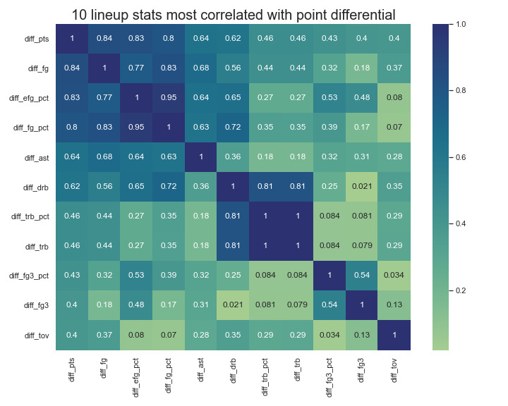
Do higher paid lineups perform better than lower paid ones? To compare the salaries of lineups across different years requires normalizing each lineup salary relative to its own year. After dropping lineups that included players that do not have salary information in the player dataset, I computed the total player salary of each lineup, league salary mean and standard deviation for the given year, and the salary z-score for each lineup.
\[Z = \frac{x-\mu_{year}}{\sigma_{year}}\]
Code
def get_lineup_salary(lineup, df_players):
    player_ids = lineup['player_ids'].split(', ')
    year = lineup['year']
    total_salary = 0
    for pid in player_ids:
        player = df_players[(df_players['year']==year) & (df_players['player_id']==pid)]
        total_salary += player['salary'].item()
    return total_salary

def get_salary_zscore(lineup, yearly_salary_mu_sigma):
    year = lineup['year']
    mu, sigma = yearly_salary_mu_sigma.loc[year].values
    return (lineup['total_salary'] - mu) / sigma

# df5 is the 5-player lineup dataset
yearly_mu_sigma = df5.groupby('year')['total_salary'].agg(['mean', 'std'])
df5['total_salary'] = df5.apply(lambda lineup: get_lineup_salary(lineup, df_players), axis=1)
df5['salary_zscore'] = df5.apply(lambda lineup: get_salary_zscore(lineup, yearly_mu_sigma), axis=1)
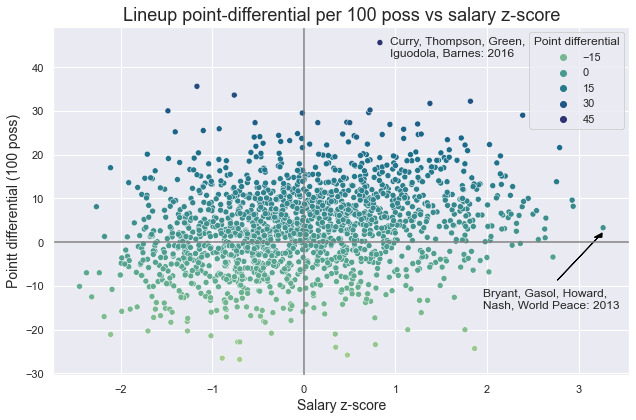
A high lineup salary does not directly indicate high performance. However, there are several factors clouding this analysis of lineup salary and performance. The 150 minute threshold likely weeds out many poor performing lineups, as teams that want to win move on quickly from terrible lineup combinations, producing a strong bias towards better lineups accumulating more minutes. Opposite this minutes bias there are several reasons organizations play bad expensive lineups on purpose: allow young players to mature, improve draft odds by losing, and the ability to acquire future assets by taking on bloated contracts from teams that want to win now.
5.4. Predicting lineup point differentials
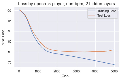
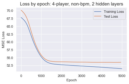
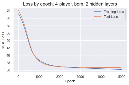
With the lineup cluster profiles as inputs, I trained several simple artificial neural networks to try and predict the observed lineup point-differentials per 100 possessions. Each fully-connected feed-forward network takes in a 12 dimensional input (the cluster profile), outputs a scalar representing the predicted point differential for the lineup, and is trained to minimize the mean-squared error of predictions vs observed point-differentials.
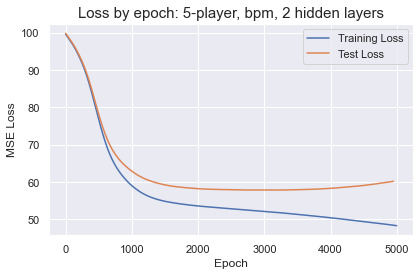
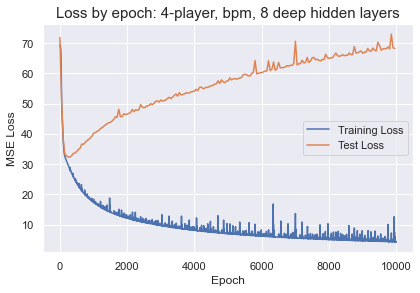
Within 2,000 epochs the test loss for every network plateaued before rising due to overfitting. Deeper networks only accelerated the learning and overfitting, with no performance improvements over a small network with 2 hidden layers and 24 units in each. The best results were obtained training on 4-player lineups with bpm-weighted cluster profiles. The predictions by the best performing networks are not going to make anyone rich betting on the NBA. The MSE translates to an average error around 5.6 points per lineup, a wide margin that is enough to distinguish solid from terrible or great from good lineups. There does not appear to be enough information in the cluster profiles to accurately predict lineup success in the NBA.
Pytorch helper functions
from sklearn.model_selection import train_test_split
import torch
import torch.nn as nn


def build_MLP(sizes, activation, output_activation=nn.Identity):
    layers = []
    for i in range(len(sizes)-1):
        active_fn = activation if i < len(sizes) - 2 else output_activation
        layers += [nn.Linear(in_features=sizes[i], out_features=sizes[i+1]), active_fn()]
    mlp = nn.Sequential(*layers)
    return mlp

def torch_train_test_split(X, y, test_size, random_state=3):
    X_train, X_test, y_train, y_test = train_test_split(X, y, test_size, random_state)
    datasets = []
    for dataset in [X_train, X_test, y_train, y_test]:
        datasets.append(torch.tensor(dataset.to_numpy(), dtype=torch.float32))
    return datasets
Train network to predict lineup success
### Load data
df5 = pd.read_csv('../datasets/master_5man_lineup_clustes_2000_2020.csv', index_col=0)
cluster_bpm_cols = [f'cluster_{n}_bpm' for n in range(12)]
cluster_nonbpm_cols = [f'cluster_{n}' for n in range(12)]

X5 = df5[cluster_cols]
y5 = df5['diff_pts']
X_bpm5 = df5[bpm_cluster_cols]
y_bpm5 = df5['diff_pts']

### Setup network, learning rate, inputs, labels,  etc.
input_dim = [12]
hidden_sizes = [24, 24]
output_dim = [1]
sizes = input_dim + hidden_sizes + output_dim
activation = nn.ReLU
mlp = build_MLP(sizes, activation)
mlp_learning_rate = 0.0001
loss_fn = nn.MSELoss()
optimizer = torch.optim.Adam(params=mlp.parameters(), lr=mlp_learning_rate)
epochs = 5000
test_interval = 50
X_train_tensor, X_test_tensor, y_train_tensor, y_test_tensor = torch_train_test_split(X5, y5, 0.2, seed)
training_losses, test_losses, test_epochs = [], [], []

### Training loop
for epoch in range(epochs):
    optimizer.zero_grad()
    y_hat = mlp(X_train_tensor)
    train_loss = loss_fn(y_hat.reshape(-1), y_train_tensor)
    training_losses.append(train_loss.item())
    train_loss.backward()
    optimizer.step()

    ### Evaluate on test set
    if epoch % test_interval == 0:
        test_epochs.append(epoch)
        with torch.no_grad():
            y_hat_test = mlp(X_test_tensor)
            test_loss = loss_fn(y_hat_test.reshape(-1), y_test_tensor)
            test_losses.append(test_loss.item())

### Plot training results:
fig, ax = plt.subplots()
train_plot = sns.lineplot(x=[i for i in range(epochs)], y=training_losses, label='Training Loss', ax=ax)
test_plot = sns.lineplot(x=test_epochs, y=test_losses, label='Test Loss', ax=ax)
ax.set_title('Loss by epoch: 5-player, non-bpm, 2 hidden layers', fontsize=15)
ax.set_ylabel('MSE Loss')
ax.set_xlabel('Epoch')
plt.tight_layout()
plt.legend();
| players | count | mean point-diff | std point-diff | non-bpm MSE (\(\sqrt{}\)) | bpm MSE (\(\sqrt{}\)) |
|---|---|---|---|---|---|
| 5 | 1,682 | 3.352 | 9.439 | 79.959 (8.94) | 57.851 (7.61) |
| 4 | 5,222 | 3.104 | 7.701 | 53.479 (7.31) | 31.729 (5.63) |
For fun we can try bigger networks and watch the network quickly overfit and memorize the training set:
input_dim = [12]
hidden_sizes = [24, 256, 512, 512, 512, 256, 24]
output_dim = [1]
6. Wrapping Up
The initial motivation for this project was to improve the current taxonomy of player types in NBA conversations. The clustering results do provide much more context than the 5 traditional positions, but they are far from an ideal positional hierarchy. To improve on my approach in the future, I would find a more robust way to separate out playing style from effectiveness. Having distinct axes of style and effectiveness would allow for a cleaner comparison between players of similar roles, as well as between the relative value of different styles with respect to team and lineup success. I think predicting lineup success with accuracy within a couple of points is difficult and I would pursue a regression based on the lineup's player stats from recent seasons, league stats from recent seasons, and historical league trends, as opposed to a regression based solely on player type; there is too much variation across individual players to rely on labels like the cluster profiles I used.
The next NBA project I work on will probably revolve around NBA player-tracking data. There are many cool possibilities; estimating possession outcomes in real-time, isolating patterns of good and bad possessions, player/coach/league evolution across several seasons. We'll see!
Footnotes:
Kevin Durant exposes his burner habit in 2017 and defends it in 2020.
Game of Zones roasts Bryan Colangelo for his horde of twitter burners.
The bottom 14 teams in each NBA season enter into a lottery for draft position. Lower ranking teams have increased odds of better draft positions. In the current system the bottom three teams each have a 14% of receiving the 1st overall selection. The structure of the lottery is the source of much discussion (re: tanking) as it figures prominently in the destiny of teams, especially given how star dependent success in the NBA is.
On basketball reference a player id is built with the first 5 characters of the players last name, first two characters of the first name, and two numbers to differentiate duplicate name codes. For example, Allen Iverson's player id is "iversal01" and Wesley Mathews is "matthwe02" given that his father, Wes Mathews, already occupies the "matthwe01" id.
This tool was convenient for gathering biographical data but was not capable of providing accurate season statistics in the categories I was looking for. Here is the documentation. It is also slow fetching data, but I can imagine using it again for different tasks.
86.84% of player-seasons have a maximum cluster probability greater than or equal to 90%.
The NBA has a soft salary cap that limits the amount that teams can spend each year. Teams that spend beyond the salary cap must pay"luxury tax" payments that escalate quickly as well as suffer restricted access to free agent players who are in the market for new contracts. Managing current and future "cap space" is a primary focus of NBA front offices. The cap and related rules are outlined in the collective bargaining agreement.